Risk Controlled Audit : Report on Daljit's Coefficients

Introduction

Section 1 reproduces the data and the plot you sent me, just so that you can be reassured that we are on the same page to start off with

Section 2 attempts to answer the questions you raised in the email

Section 3 My preferences and suggestions

Section 4 shows data in groups of 116 in case you want to look at them

Section 5 Summary and remarks

Section 1 : Data you sent

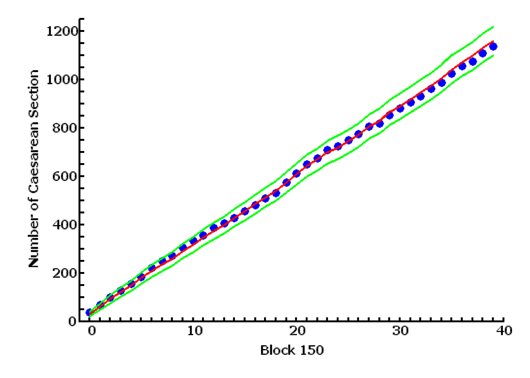
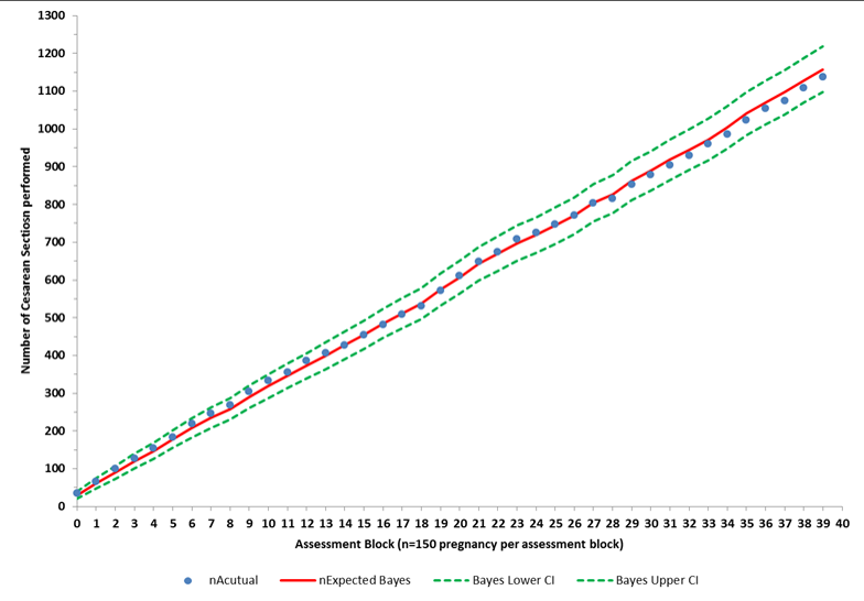
The table that follows, table 1.1, is copied from your email,and reproduced here. The only change is that I have used 4 decimal point precision for all values other than counts

The two plots, fig. 1.1 and 1.2 reproduced the plot you sent me. The one on the left, 1.1 is produced by me from the data in table 1.1, and the plot on the right is copied directly from your email. The two plots are the same except for slight differences in color, dot size, and line thickness.

At this point, we can be reassured that we are discussing the same data

Section 2 : Respond to your suggestions in the email

For our purposes we are proposing that actual rates be compared against a comparator in order to tests deviation from expected. Can you calculate a few more things

1) sum up probs for all pregnancies in each year by model as this would be expected number of CS and an estimate as to overall under or over estimate

2) Can you break down data in 2014 to determine the distribution of the difference between actual and observed CS rates. We could then use this to determine how large a difference we aim to detect in CUSUM. Alternative is to keep it simple and plot chart something like one below which shows the cumulative number of actual and expected number of CS by consecutive block with an estimate for the 95% CI of the estimate using n* (p+/- 1.96*SQRT(p(1-p)/n)) where p is the proportion of expected CS .

The following table, 2.1. attempts to answer 1). Please note that 95% confidence intervals are calculated as mean ±1.96SE, and SE=sqrt(p(1-p)/n), and p = number of caesarean section /total births

	2014	2014
Number of births in the study	6038	6038
Number of caesaren sections	1145	1220
Caesarean section rate(95%CI)	0.190(0.180 to 0.199)	0.202(0.192 to 0.212)
Mean naïve Bayes Probability(95%CI)	0.185(0.175 to 0.195)	0.189(0.179 to 0.199)
Mean logistic regression probability(95%CI)	0.183(0.173 0.193)	0.177(0.167 to 0.187)

Table 2.2. tanslates table 2.1. into actual and estimated number of caesarean sections by multiplying probability to the number of births

	2014	2014
Actual number of Caesarean sections(95%CI)	1145(1085.1 to 1204.5)	1120(1158.8 to 1281.2)
Naïve Bayes estimated number of Caesarean sections(95%CI)	1117.0(1057.9 to 1176.2)	1141.2(1081.6 to 1200.8)
Logistic regression estimated number of Caesarean sections(95%CI)	1105.0(1046/1 to 1163.8)	1068.7(1010.6 to 1126.9)

Table 2.3. answers 2), and shows the difference (actual-expected) in each group

Summary of the difference are :

n = 40, minimum = -22.0, maximum = 15.5
mean = -0.8, Standard Deviation = 11.1, Standard Error of Mean = 1.8
95% CI of group means = -22.6 to 20.9, 95% CI of yearly mean = -4.3 to 2.7
Skewness = -0.4346, Standard error = 0.3873, 95% CI = -1.1937 to 0.3246
Kurtosis = -1.1199, Standard error = 0.7746, 95% CI = -2.6381 to 0.3983
Median = -0.5
Median-Mean = -0.3, Standard error = 1.8, 95% CI = -3.9 to 3.3

The mean difference is 0.8, less than 1, and the 95% confidence interval for the mean is -4.3 to 2.7 out of groups of 150, or -2.9% to 1.8%.

The plot of the differences in each group from 2014 are shown in fig 2.1

I understand your approach to determine what difference we should try to detect. It is based on laboratory protocols. Firstly you determine the normal range, then you define the abnormal as anything outside the normal range. However, auditing is a different situation, and such an approach have problems.

Firstly these figures are precision figures. They are useful to determine the normal range in a measurement, or in a research setting, to determine the critical difference and sample size of your research model thay are likely to yield a statistically significant result. The approach you suggested is however not appropriate to determine the difference to detect in an audit, as this is a clinical and not a statistical decision, based on why the audit is done and the difference to detect is one that indicates a need for investigation and remedy

Secondly, statistically setting a critical difference (effect size) to detect presupposes that this effect size and the inter-relationship between all variables in the model are invariant. The reason for doing an audit is because we suspect things are not invariant, and when changes come we want to know.

Thirdly, choosing a difference in this manner is too specific, as it is based on the binomial distribution with a caesarean section rate of around 19% and a group size of 150. As you know, variance (standard error and hence 95% confidence interval) in binomial distribution is highly sensitive to the proportion being study and to the sample size. This means that the results we obtained would be difficult to generalize.

Fouthly, in an audit, we are not trying to detect a group that is a statistical outlyer, but to detect a changing trend. this means that a single or even a small cluster of significant departures are not meaningful. To detect a changing trend means to detect very small but persistent changes as quickly and surely as possible. The difference we are trying to detect is not that one or a small cluster of groups are significantly different to the expected, but that there is a persistent change away from the expected, even very small ones.

Fifthly, your thinking is based on hypothesis testing based on Type I and II errors. These probabilities are based on a single set of observations, and interpreting repeated sets requires either a Bonferoni's correction or more complex meta-analysis type of analysis. An audit is really a time series study, representing frequent and repeated sets of observations where the sets are likely to be auto-correlated. Our data are actually 40 such sets of 150 cases in each set. The probabilities involved are therefore much more complex than that in a single set of data.

Section 3 : My preferences and suggestions

I am learning a lot and enjoying myself enormously looking at the data one way and another, and debating with you on the pros and cons and how to proceed. I feel that, at my stage of life, it is a real privilege to be able to work with someone like you, and having such detailed and relaxed discussions. I therefore do not feel strongly about any aspect of this project. If you feel strongly about anything, I will go along even if I disagree with you (after a bit of argument first). This of course applies to our current discussions.

However, I am assuming that you are equally relaxed and tolerant to my opinions, and in response to your email I would like to suggest the following for you to consider.

Using groups of 150 is OK as it is large enough. Can I recommend however that we use groups of 116 instead, as this has two advantages. Firstly this gives us 52 instead of 40 groups a year, providing greater sensitivity in an audit while the group standard deviations would not be all that different to 150 at this level. Secondly, it is intuitively easier to understand, as this represent auditing at a weekly interval, when all the variations in the workload are evened out, and the audit fits in with the routines of clinical supervision

I recommend that we avoid the binomial distribution because of its sensitivity to the sample size used and the proportion being considered. We should create indeces, such as departure from benchmark (group caesaresn section rate - 0.19), changing risks (group mean probability estimates - 0.19), and caesarean section rate in excess of risks (group caesarean section rate - group mean probability estimates). We should then test these indecis against normal distribution as I have done in Report 1b, and once demonstrated that we can assume them to be normally distributed, use them as such. This would give us flexibility in using the data and have a greater range of statistical procedures available to us. The normal distribution is also more familar to most clinicians so our paper would be easier to understand. We will have less lengthy explanations.

I would like to suggest that we abandon using statistical criteria to determine the change we wish to detect. This approach is cumbersome, difficult to understand by the uninitiated, and requires a lot of explanation. Can I suggest that we approach it clinically, and decide that we wish to detect a change of 1%, and in a reasonably short time (a few months) if it happens. Caesarean sections are continuing to increase, by about 1% a year. Obstetricians are obsessed about the percentage and not actual numbers as percentage is corrected for different sample size so it is easier to compare. A change of 1% within a year is therefore meaningful to most clinicians and quality controllers. However a difference of 1% is so small and variations in caesarean section rates are so great that normal inferential statistics would have difficulty to detect it, and quality controllers will need some auditing approach such as CUSUM to detect it, one of the points we try to make in our paper.

I still think we should use CUSUM for continuous monitoring as this is the standard in quality control, and also the results I have produced in Report 1b looked good. However, if you do not like it we can explore an alternative I think you are more familiar with. We can do exponentially weighted moving averaging (EWMA). This is easier to do, have less theoretical statistic presumptions, and because it is used extensively in the stock market, it is more familar to and intuitively easier to understand by the clinicians. I recalled that you used EWMA to even out the electronic signals in fetal ECG, and tried in vain to make me understand it. I have now understood it and have provided programs and explanations on the department's web site in case you want to look at it. If you want to explore this (even if you have not decided to use it) please let me know and I will put our data on it. The url are http://www.obg.cuhk.edu.hk/ResearchSupport/StatTools/EWMA_Pgm.php for the program and http://www.obg.cuhk.edu.hk/ResearchSupport/StatTools/EWMA_Exp.php for my explanations.

Section 4 : Groups of 116

Table 4.1. contains 52 groups of 116 consecutive births from 2014, with group mean caesarean section rates and group mean Bayes probability. If you decide to accept my recommendations and use it, I can provide group means for logistic regression as well, and for both 2014 and 2015.

Fig.4.1. is a plot of difference between group caesarean section rate and group mean Bayes probability for 2014, using gtoups of 150 birthe. Fig.4.2. is the same plot, but used groups of 116 births. The two have the same scale for comparison.

Fig.4.3. have the two plots superimposed on top of each other, red for groups of 150 and blue for groups of 116.

It can be seen here that using rate rather than count, comparisons are more flexible as sample size is already corrected for.

The greater number of smaller groups, block 116, does have greater variations, but the patterns from the two size groups are very similar.

Section 5 : Summary and concluding remarks

• I suggest groups of 116 rather than 150
• I suggest that we use an increase of 1% as the critical change to detect, arguing from the clinical and auditing perspective rather than basing it on what statistically can be detected
• I suggest abandoning references to binomial distribution. Instead we should create indeces and test them for normal distribution. Once normal distribution is demonstrated, we should use the indeces for auditing using parametric statistics methods
• I still prefer CUSUM for continuing monitoring, but suggested EWMA is a good alternative if you think CUSUM too cumbersome.